The Hesitation

Suppose I want my chatbot to be conservative in its learning, what are the ways we control that? There is dropout, and weight decay, and normalization. One idea was to find a way for it to learn and then sleep for a while before learning again. If we look at the gradient of such a function, it would look like $1+ cos(x)$ :

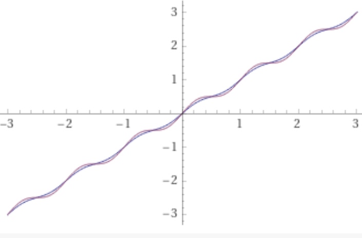
This gradient is motivated by the want of rest period, when the input passes a certain periodic magnitude the progress of gradient based optimizer is gradually slowed down(but still pointed towards the same direction.) After the sleep, the function wants to progress fast to make up for the time spent sleeping, so the steps are bigger. A bit of manipulation of that expression produces the function with that gradient function $x+sin(x)$

This addition of a hesitation can be used as a foreactivation (defined in previous FAM entries). Or in fact the hesitation layer can be placed any where a dropout is normally used.

A certain amount of experimentation is required to inject useful amount of randomization. This layer is particularly easy to instantiate after units that have known scaling, such as sigmoidal activations, softmax, batchnorm, and others. One formula in particular is amplitude. For $\alpha \in (0, 1]$ The hesitation layer $H_\alpha(t) = t + \alpha sin (2 \pi t)/{2\pi}$ makes it possible to adjust the flat part of the sleep cycle. Here is $\alpha = 0.5$ in blue next to the original:

$H_{\alpha=0.5}(t) = t + \alpha sin (2 \pi t)/{2\pi}$

More work is needed to establish the precise effect this layer has different types of optimizers. For optimizers like Adam, the added variability would normally increase the noise of the gradients passing through the layer thereby effecting a reduction the learning rate. For $\alpha>1$ the hesitation layer becomes non-monotonic, but since Adam accumulates gradients, the gradient in the “wrong” direction will slow the progress of optimization more significantly than smaller $\alpha$ ’s. It will not necessarily produce an unrecoverable valley of local minimum. For $\alpha \in (0, 1)$ this layer will not introduce new univariate local minimums or saddles to the optimization it is being added to. With randomization, the units will sleep at different times giving other paths of gradient that are not sleeping a chance to explore their potential to improve.

Another direction to explore is learnable sleep cycles in the form of $H_{\alpha\beta}=x + \alpha sin(2 \pi \beta x)/{2 \pi \beta}$ . Where $\alpha \beta$ are either a single scalar or properly sized tensor for element-wise application. Generally the adjustment of $\alpha \beta$ will be for quicker progress towards the direction of underlying gradients.

Wdyt?

Ps one can work out the gradient $H_{\alpha}(f(x))= f(x) + \alpha sin(f(x))$ . Take the derivative wrt $x$ . $\partial H_{\alpha}(f(x)) / \partial x= (1+\alpha sin(f(x))\partial f(x)/ \partial x$ . So you see the gradient varies between $[1-\alpha, 1+\alpha]$ times of $f(x)$ ’s gradients.